Telecoms - Display Cell Tower KPIs in Icon Map Pro

A common use case for our telecoms customers is to show cell tower locations, using wedge diagrams, to represent various information and KPIs. This blog shows a repeatable approach for achieving this using Icon Map Pro.
Consider our source data:
| SiteID | CellID | Latitude | Longitude | Azimuth | Beamwidth | Throughput |
|---|---|---|---|---|---|---|
| SITE_1 | CELL_1_2 | 51.5104471707975 | -0.143399762 | 0 | 65 | 10 |
| SITE_1 | CELL_1_2 | 51.5104471707975 | -0.143399762 | 90 | 65 | 10 |
| SITE_1 | CELL_1_3 | 51.5104471707975 | -0.143399762 | 180 | 90 | 6 |
| SITE_1 | CELL_1_4 | 51.5104471707975 | -0.143399762 | 270 | 90 | 6 |
| SITE_2 | CELL_2_1 | 51.519405119581 | -0.113691529 | 0 | 45 | 10 |
| SITE_2 | CELL_2_2 | 51.519405119581 | -0.113691529 | 90 | 90 | 10 |
| SITE_2 | CELL_2_3 | 51.519405119581 | -0.113691529 | 180 | 45 | 6 |
| SITE_2 | CELL_2_4 | 51.519405119581 | -0.113691529 | 270 | 45 | 6 |
| SITE_3 | CELL_3_1 | 51.5178896481135 | -0.147332693 | 0 | 60 | 10 |
| SITE_3 | CELL_3_2 | 51.5178896481135 | -0.147332693 | 90 | 60 | 10 |
| SITE_3 | CELL_3_3 | 51.5178896481135 | -0.147332693 | 180 | 90 | 6 |
| SITE_3 | CELL_3_4 | 51.5178896481135 | -0.147332693 | 270 | 90 | 6 |
| SITE_4 | CELL_4_1 | 51.5086784040137 | -0.132543639 | 0 | 65 | 10 |
| SITE_4 | CELL_4_2 | 51.5086784040137 | -0.132543639 | 180 | 65 | 6 |
| SITE_5 | CELL_5_1 | 51.5072231988425 | -0.140595659 | 0 | 60 | 10 |
| SITE_5 | CELL_5_2 | 51.5072231988425 | -0.140595659 | 120 | 45 | 10 |
| SITE_5 | CELL_5_3 | 51.5072231988425 | -0.140595659 | 240 | 65 | 6 |
| SITE_6 | CELL_6_1 | 51.5161939797486 | -0.126133127 | 0 | 90 | 6 |
| SITE_6 | CELL_6_2 | 51.5161939797486 | -0.126133127 | 120 | 60 | 6 |
| SITE_6 | CELL_6_3 | 51.5161939797486 | -0.126133127 | 240 | 90 | 6 |
We have 6 sites, each with a number of sectors (cells), located using latitude and longitude. Each sector has its azimuth (the central pointing direction of the antenna, measured clockwise from true north) and its beamwidth (the angular width of the main lobe). We also include the current throughput KPI for each cell. We’re going to use this throughput value to drive the wedge coloring.
To show the wedge symbols for each site, we're going to construct an SVG for each location. This is a great opportunity to use a new feature in Power BI - DAX User Defined Functions (UDFs). However, at the time of writing, this is a preview feature, so we need to ensure it's enabled in Power BI's preview features settings:
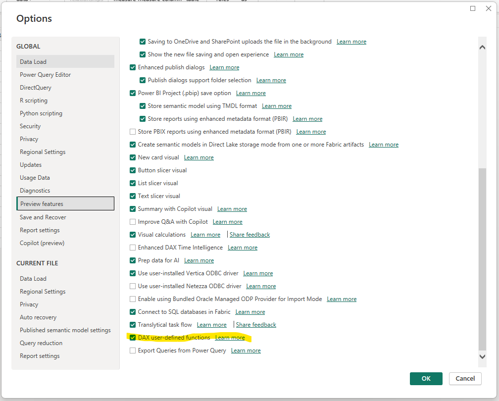
You will need to restart Power BI Desktop after enabling this feature.
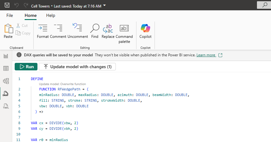
With this enabled, we can now use Power BI's DAX view to paste in our UDFs.
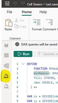
Our main UDF generates a single wedge as an SVG path. We also have a couple of other functions to ensure our SVG is rendered correctly as a data URL to include in the map.
DEFINE
    FUNCTION RFWedgePath = (
    minRadius: DOUBLE, maxRadius: DOUBLE, azimuth: DOUBLE, beamWidth: DOUBLE,
    fill: STRING, stroke: STRING, strokeWidth: DOUBLE,
    vbw: DOUBLE, vbh: DOUBLE
  ) =>

VAR cx = DIVIDE(vbw, 2)
VAR cy = DIVIDE(vbh, 2)

VAR r0 = minRadius
VAR r1 = maxRadius

VAR a0 = azimuth - beamWidth / 2
VAR a1 = azimuth + beamWidth / 2

VAR rad0 = RADIANS(a0)
VAR rad1 = RADIANS(a1)

VAR x0o = cx + r1 * COS(rad0)
VAR y0o = cy - r1 * SIN(rad0)
VAR x1o = cx + r1 * COS(rad1)
VAR y1o = cy - r1 * SIN(rad1)

VAR sweep    = 0
VAR largeArc = IF( ABS(a1 - a0) > 180, 1, 0 )

VAR dPath =
    IF(
      r0 <= 0,
      "M " & NumText(x0o) & " " & NumText(y0o) &
      " A " & NumText(r1) & " " & NumText(r1) & " 0 " & largeArc & " " & sweep & " " &
             NumText(x1o) & " " & NumText(y1o) &
      " L " & NumText(cx)  & " " & NumText(cy) & " Z",
      VAR x1i = cx + r0 * COS(rad1)
      VAR y1i = cy - r0 * SIN(rad1)
      VAR x0i = cx + r0 * COS(rad0)
      VAR y0i = cy - r0 * SIN(rad0)
      RETURN
      "M " & NumText(x0o) & " " & NumText(y0o) &
      " A " & NumText(r1) & " " & NumText(r1) & " 0 " & largeArc & " " & sweep & " " &
             NumText(x1o) & " " & NumText(y1o) &
      " L " & NumText(x1i) & " " & NumText(y1i) &
      " A " & NumText(r0) & " " & NumText(r0) & " 0 " & largeArc & " " & (1 - sweep) & " " &
             NumText(x0i) & " " & NumText(y0i) & " Z"
    )

RETURN
  "<path d='" & dPath & "' fill='" & fill & "' stroke='" & stroke &
  "' stroke-width='" & NumText(strokeWidth) & "' />"

DEFINE
    FUNCTION NumText = (n: DOUBLE) =>
VAR t = FORMAT(n,"0.########")
RETURN IF(RIGHT(t,1)=".", LEFT(t,LEN(t)-1), t)


DEFINE
    FUNCTION UrlEncodeSvg = ( raw : STRING ) =>
    SUBSTITUTE(
        SUBSTITUTE(
            SUBSTITUTE(
                SUBSTITUTE(
                    SUBSTITUTE(
                        SUBSTITUTE(
                            raw,
                            " ", "%20"
                        ),
                        "#", "%23"
                    ),
                    """", "%22"
                ),
                "<", "%3C"
            ),
            ">", "%3E"
        ),
        "'", "%27"
    )
Paste this into the DAX query window and press the "Update model with changes (3)" button.
We now have a reusable set of functions that we can call from inside a DAX measure.
However, before we generate our tower SVG, we're going to create a quick DAX measure to determine the wedge colors based on the Throughput value.
Add the following measure:
KPI Color =
VAR t = SELECTEDVALUE('Cells'[Throughput])
RETURN
SWITCH(
    TRUE(),
    ISBLANK(t),              "#BDBDBD",   -- no data: grey
    t <= 2,                  "#d73027",   -- red
    t <= 4,                  "#fc8d59",
    t <= 6,                  "#fee08b",
    t <= 8,                  "#d9ef8b",
    t <= 10,                 "#91cf60",
                              "#1a9850"   -- >10: green
)
Now we're ready to add our measure to generate the SVGs. This measure will aggregate the cells belonging to a site and generate a combined SVG symbol for that site:
Site Symbol =
VAR width       = 300
VAR height      = 300
VAR strokeColor = "#000000"
VAR strokeWidth = 4
VAR minRadius   = 18
VAR maxRadius   = 140

VAR paths =
    CONCATENATEX(
        'Cells',
        RFWedgePath(
            minRadius, maxRadius,
            'Cells'[Azimuth],
            'Cells'[Beamwidth],
            [KPI Color],
            strokeColor, strokeWidth,
            width, height
        ),
        ""
    )

RETURN
"data:image/svg+xml;utf8," &
UrlEncodeSvg(
    "<svg xmlns='http://www.w3.org/2000/svg' viewBox='0 0 " & NumText(width) & " " & NumText(height) & "'>" &
      paths &
    "</svg>"
)
It generates a series of paths, one for each cell, and then wraps them up in an SVG tag. We then use our new UrlEncodeSvg function to URL Encode the SVG and create it as a data URL.
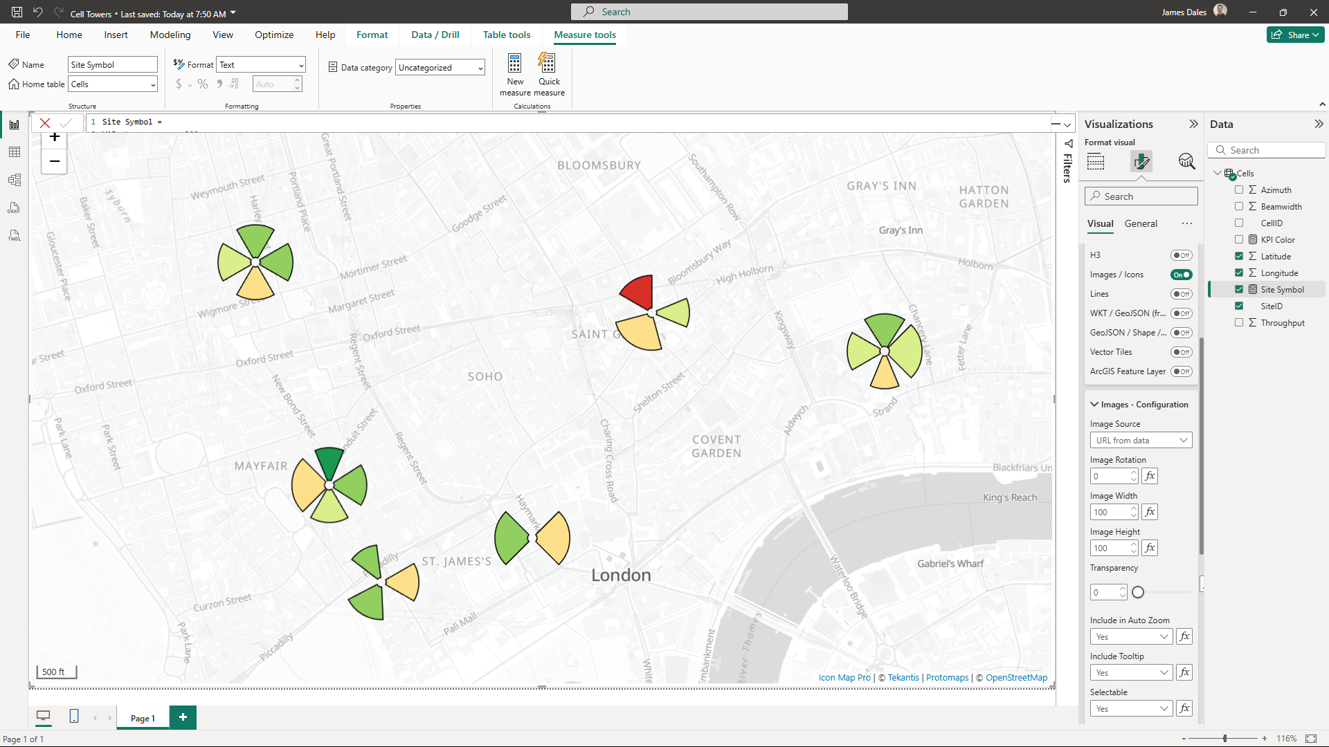
We're now ready to configure Icon Map Pro to show our cell tower locations.
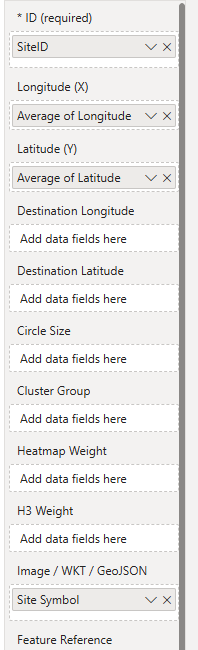
The data configuration is straightforward. The ID field in Icon Map Pro should represent the granularity of each item we want on the map, which in this case is a cell tower site, so add the Site ID to Icon Map Pro's ID field. Then drag in the longitude and latitude. Ensure the aggregation type is Average. This will make sure the longitude and latitude stays the same for each site. Then drag our new Site Symbol measure to the Image / WKT field:
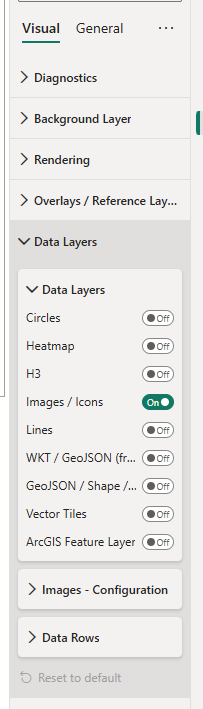
The final step is to turn on the Image Data Layer in Icon Map Pro's settings:
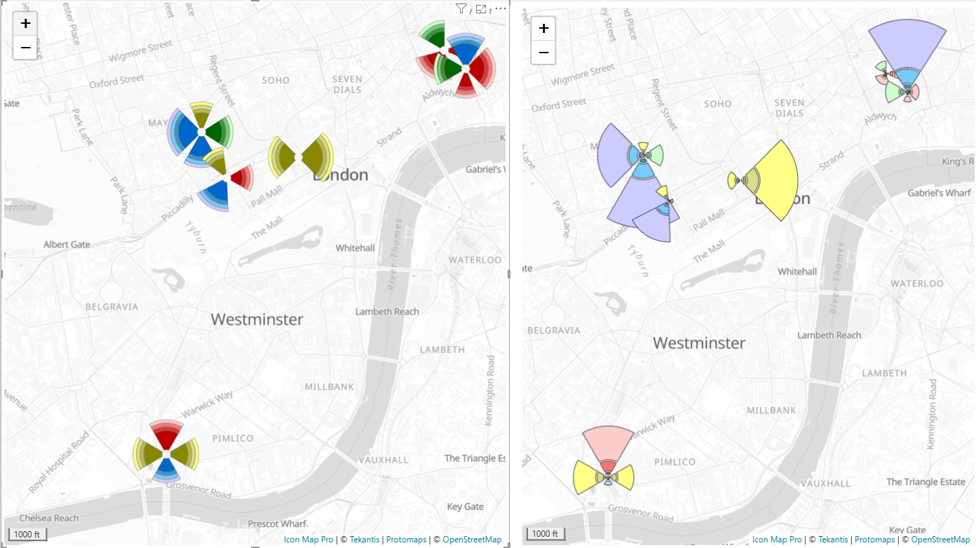
Your map should now look like this:
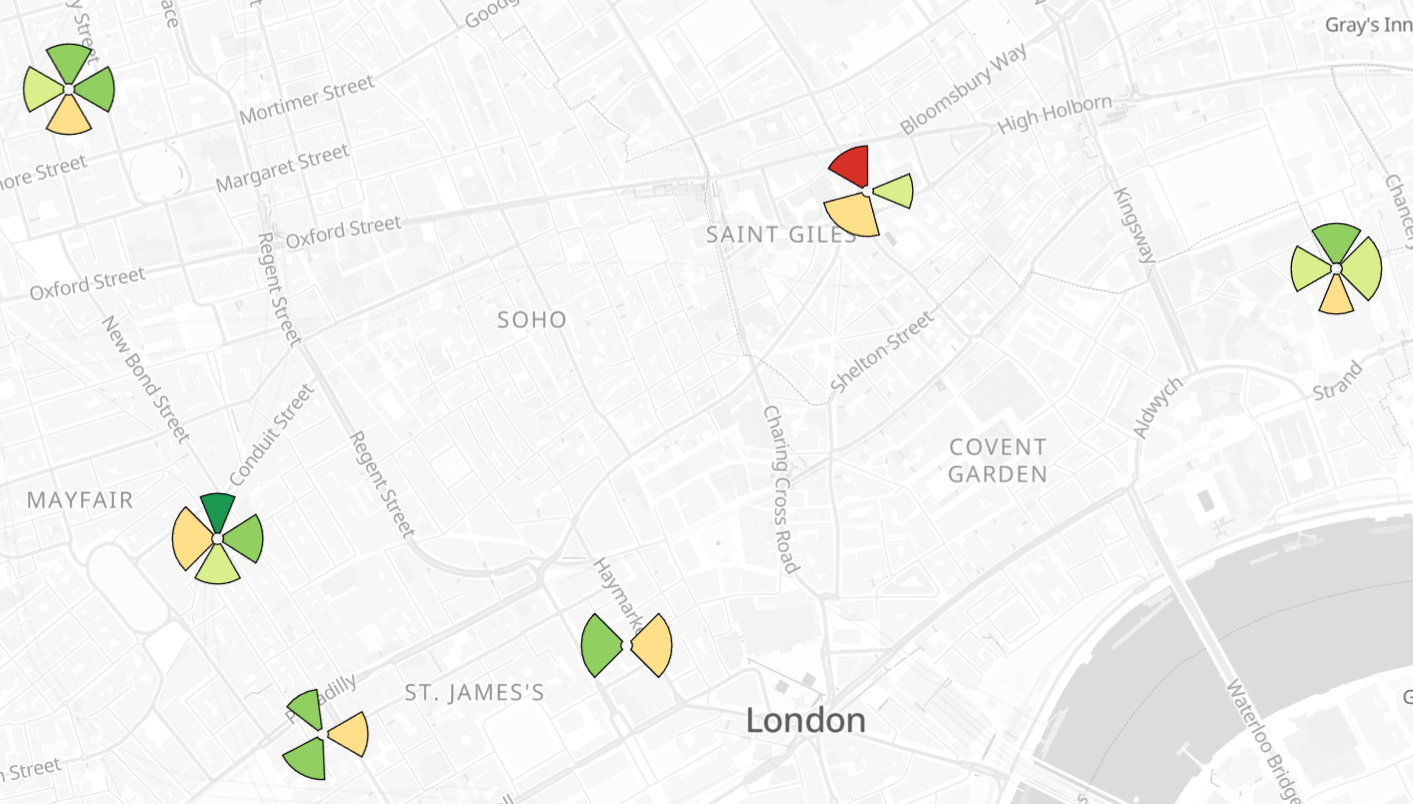
You can download the .pbix file to see this in action.
These same functions can be used to draw more complicated diagrams by varying the min and max radius settings: